Mars Lander

Play the online demo here

This second article continues on from the first article in which I covered the web-based simulator, graphics, and terrain generation. In the this article we’ll cover the landing autopilot, and how I used a Darwinian inspired machine learning approach called genetic algorithms to optimise its parameters.

The Autopilot

We’ve seen a semi-realistic Martian spacecraft built to run in web browser, but as you may have found if you’ve tried running in browser yourself, it’s really really hard to land. Actually - the required threshold of maximum $1\text{m/s}$ normal and surface velocity set by the professor for this coursework was very unforgiving and made it nearly impossible to land by hand!

Enter control theory. If we have the ability to set the direction and throttle of the craft, and assume perfect access to position and velocity, perhaps we can design some function $f(\bf{x}, \dot{\bf{x}})$ that sets the throttle, such that our Mars Lander lives up to its name, and isn’t a Mars crash- Lander.

By the way - assuming perfect access to position and velocity is a big assumption, quite a few expensive space craft have been lost because of failures with velocity and/or position sensors. In December 1999, spurious signals from a magnetic sensor caused NASA’s Mars probe to detect that it had landed and shut off it’s engines, when it was still $40\text{m}$ above the surface and travelling at $>10\text{m/s}$¹. In April 2023, Japan’s moon probe detected it had landed, when it was still $5 \text{km}$ above the surface, due to an failure case triggered by passing over the rim of a crater².

Control Theory

So how can we design a control function to set the throttle? This is a classic control theory problem, and whilst we were taught in much more detail about the ins and outs of transfer functions and block diagrams as we went through IB Engineering, this was our first introduction. The equations for the autopilot were explained and given in a handout³ which I’ve based the following description closely upon.

Let’s start with some basic first principles and design an autopilot function from that. For simplicity we’ll say $h$ is the height relative to the Martian surface and $\dot{h}=\frac{dh}{dt}$ is the vertical velocity (in the actual simulation, we have to take dot products with the surface normal vector). Then how can we design a function $f$ that sets the throttle between 0 and 1 based on $h, \dot{h}$?

Suppose our strategy is that the descent rate should decrease linearly as the lander approaches the surface,

$$ \dot{h} = -(0.5 + K_h h) $$

where $K_h$ is a positive scaling constant. We can easily sense check this; being on the surface is $h=0\text{m}$ so gives $\dot{h}=-0.5\text{m/s}$, which is a gentle descent of $0.5\text{m/s}$ and within the $1\text{m/s}$ requirement. If we’re $1\text{km}$ up, and with $K_h=0.01$, then $\dot{h}=-10.5\text{m/s}$ which is seems like an acceptable speed to be going downwards whilst a kilometre above the surface. So how can we set the throttle to achieve this state of affairs? Rearranging the above expression gives

$$ e = -(0.5 + K_h h) - \dot{h} $$

where $e$ is an error term which we want to keep as close to zero as possible, to maintain the strategy. We can use a simple proportional controller that sets the throttle in such a way as to keep $e$ small. Defining

$$ P_{out} = K_p e $$

where $K_p$ is another scaling constant, we can then use $P_out$ to set the throttle. If the lander is descending too quickly, then $\dot{h} > -(0.5 + K_h h)$ and $e>0$, so $P_{out}>0$, which is good, because the throttle should also be increased in this situation. Unfortunately for realism the throttle can’t be infinite or negative, and is bounded to the range $[0, 1]$, so here we diverge from linear control theory and add a parameter $\Delta$ which shifts $P_{out}$ to the correct range. I’ve pinched the following graph from the handout³.

So putting this all together, we have the following control equations;

$$ P_{out} = K_p [ -(0.5 + K_h h) - \dot{h} ] \\ \text{throttle} = \text{clamp}(P_{out}, \Delta) $$

We’ve also got a parachute we can use! This is highly nonlinear so we’ll save that for later. In the simulation, we’ll have the following configurable parameters for the autopilot:

• gain controller gain $K_p$
• kh constant for scaling altitude value $K_h$
• delta offset $\Delta$ for scaling throttle output to [0, 1]
• parachuteAltitude deploy parachute if at or below this altitude

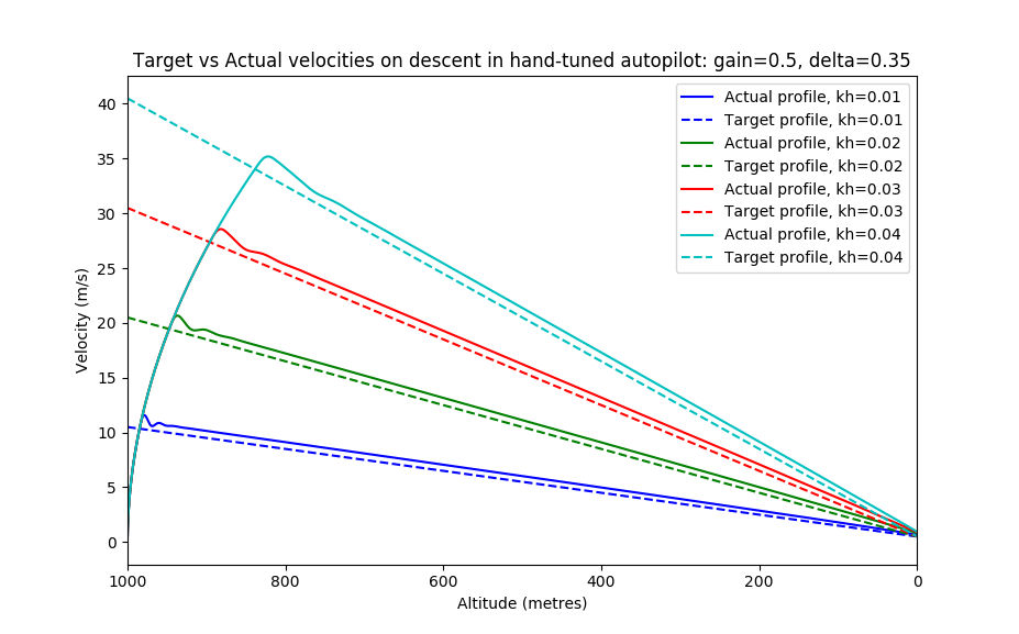
After a bit of trial-and-error parameter and values by hand, the lander was able to land safely from a basic $1\text{km}$ descent. Hooray, a functioning autopilot! But start introducing complexities of varying terrain height, atmosphere density, windspeed, a variety of different start conditions, and all the bells and whistles of the simulation from the last article, and hand-tuning becomes much harder. This begs the question: can we use the same autopilot with different parameters to solve a wider variety of scenarios?

Genetic Algorithm for Autopilot Tuning

To fine-tune the autopilot parameters, I employed a genetic algorithm implemented from scratch in JavaScript. The algorithm follows these steps:

1. Population Initialization: Generate a population of autopilots with randomly selected parameters for the PD controller (gain, kh, and delta). Parameters are initialized as 5 * Math.random().

2. Offline Simulations: Iterate through each autopilot, running (offline) simulations of landing scenarios until the lander reaches the Martian ground or a simulation-time limit is reached.

3. Scoring Autopilots: Score each autopilot based on its performance in simulations. A fitness score is computed using a chosen fitness function, depending on the optimisation goal.

4. Next Generation Creation: Create the next generation by autopilots, with offspring parameters generated by selecting values from random choices of two parents. Fitter parent autopilots are weighting up, making them more likely to be selected for reproduction. There is a chance (10%) of mutation, realised by scaling the value by a random scalar in the range [0.5, 2.0).

5. Repeat Generations: Repeat the process for several generations until the population converges to its optimum fitness.

As generations progress, the population’s fitness improves, filtering out weaker agents. The fittest individual in the last generation becomes the autopilot with parameters much improved from the manual tuning. However, the real strength of the genetic algorithm lies in its ability to optimise any arbitrary fitness function. The chosen fitness function minimises impact velocity while also minimizing leftover fuel. The programmed fitness function is as follows:

1
2
3
4
5
6
7
8
9

const descentVelocity = Math.abs(simulation.descentVelocity());
const surfaceVelocity = Math.abs(simulation.surfaceSpeed());
let fitness = 0;
fitness += (100 - Math.min(100, descentVelocity));
fitness += (100 - Math.min(100, surfaceVelocity));
if(descentVelocity <= 1 && surfaceVelocity <= 1) {
    fitness += simulation.fuel;
}
return fitness;

Fitness Scoring and Training Results

It’s crucial to note that a fitness score is only awarded for a successful landing if both lateral and vertical velocities are less than or equal to $1 \text{m/s}$, i.e. a successful touchdown. This condition alters the maxima of the fitness function to ensure prioritisation of safe landings, avoiding scenarios where the lander uses less fuel (good) at the cost of not surviving touchdown (bad).

The graph below illustrates the results of a training run, showing the mean fitness score of the entire population at each generation, normalized from 0 - 100. This particular run optimized fuel usage, training a population of 50 autopilots over 60 generations.

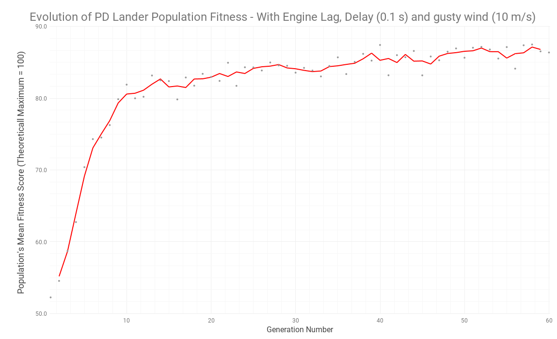
This algorithm achieved convergence in just $50 \times 60 = 300$ autopilot simulations, requiring only a minute or two of processing on a relatively low-power compute server. The fittest autopilot in the final population scored 97.8 / 100. This drastically outperforms brute force search: consider that realistic parameter values of gain, kh, delta, range four orders of magnitude from say $(0.001, 10)$, then a brute force search with ten values per decade would require $(4 \times 10)^3 = 64,000$ searches, without even matching the parameter resolution of the genetic algorithm.

The converged parameters for the fittest autopilot in this test run were as follows:

1
2
3
4
5
6

{
    gain: 2.939330,
    kh: 0.236629,
    delta: 1.111959,
    parachuteAltitude: 2614.922,
}

I tried very hard to tune my own autopilot - which did work - but despite my efforts, this genetically evoled autopilot used around 30% less fuel than mine did. A great improvement!

Taking the Genetic Algorithm Further

The versatility of the genetic algorithm becomes apparent when changing the objectives of the problem - we can solve any new problem just by adjusting the fitness function and rerunning. For example, after taking account atmospheric effects into the simulation I didn’t need to retune the parameters manually, I just ran the genetic algorithm again. This is particularly important considering the following observation: the local terrain height of the Martian surface varies, and so the density of the atmosphere on descent, varies depending on the landing spot. This has a significant impact on how much the atmosphere slows the lander down, and hand-tuned parameters may not generalise well to other landing spots. With the genetic algorithm, as long as we include this effect during training, the resulting parameters learned are a robust solution. This is a classic example of overfitting in machine learning.

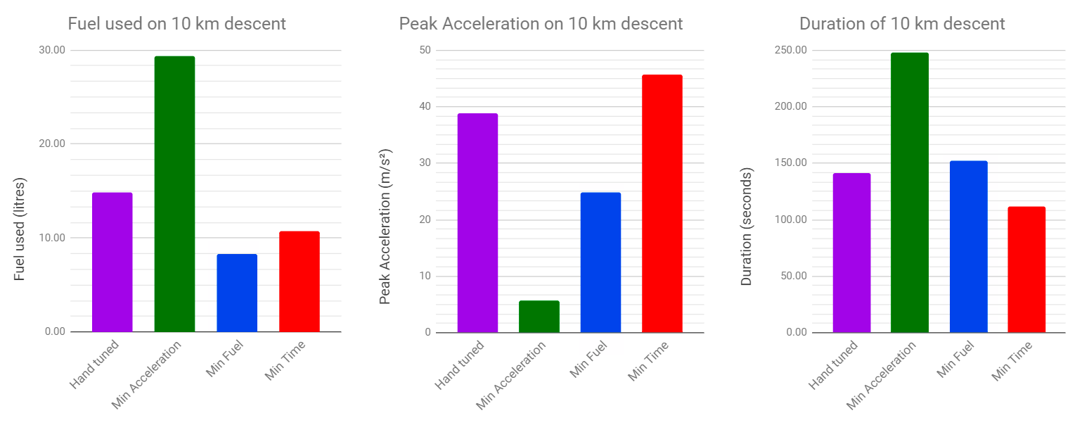
The same flexibility was clear when I tried optimising the autopilot to minimise either total descent time, or peak acceleration value. This was very easy to implement, only having to change the one following line of code. The following line from the above block,

1

fitness += simulation.fuel;

was changed, to minimise peak acceleration (improving survivability of passengers & cargo), to the following:

1

fitness += (400 - Math.min(400, simulation._maxAcceleration));

and to minimise descent time, to the following:

1

fitness += (1000 - Math.min(1000, simulation.simulationTime));

The algorithm very clearly produced a different optimum solution each time, as shown in the following figures.

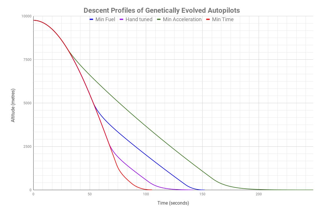
The actual final values of parameters were as follows:

 1
 2
 3
 4
 5
 6
 7
 8
 9
10
11
12
13
14
15
16
17
18
19
20
21
22
23
24
25
26
27

const handTuned = {
    gain: 0.2,
    kh: 0.1,
    delta: 0.6,
    parachuteAltitude: 3000
}
 
const minFuel = {
    gain: 3.10854,
    kh: 0.145318,
    delta: 1.80475,
    parachuteAltitude: 5343.94
}
 
const minAcceleration = {
    gain: 3.79465,
    kh: 0.0734257,
    delta: 3.28194,
    parachuteAltitude: 8452.36
}
 
const minTime = {
    gain: 0.599284,
    kh: 0.140581,
    delta: 0.646384,
    parachuteAltitude: 1741.53
}

It’s quite interesting how much the parameters do vary between the different objects. Some are not surprising, e.g. the minimum time parameters have the parachute altitude much lower. So there we have it - an autopilot that can land our craft from a variety of scenarios, inside the Mars Lander simulator, and all running inside your web browser!

Overall Summary

All in all this was a project that took rather longer and went into more depth than I originally intended. I initially set out to see if it would be possible to improve on the OpenGL software by writing it in WebGL, and started with the hardest parts of the project that I thought would be the limiting factors. It took me a good few days to sink my teeth into these problems, but by the time I’d done that I decided I was already invested in working it all the way through.

I was certainly pleased with the end result, and glad to have built on my experience in front-end development and Javascript in general. Several months after submitting, I found out that this project had won the year wide Cambridge University Engineering Department competition - “The Airbus Prize”. I was thrilled that after so much development the judges were pleased with the submission 😊. Prof. Csányi had the following kind words;

Tom’s Mars Lander project is truly outstanding. He addressed almost all of the suggested extension activities. He even wrote a genetic algorithm to evolve optimal PID autopilots for minimum fuel, acceleration or descent time. The graphics were greatly improved to furnish Mars with realistic terrain, both from a distance and also close up, with the local terrain height accounted for in the autopilot when landing. And then Tom rewrote more or less the entire code base in WebGL, so that the simulator can be run in a browser.

― Professor Gabor Csányi, Cambridge University Engineering Department